Noise shaping
Introduction
Noise shaping is a technique that is often used in combination with dithering in the context of quantization. The purpose of noise shaping is to alter the spectral shape of the error that is introduced due to dithering and quantization. Sometimes it may be desirable to concentrate most of the noise power in a certain frequency band so that the overall noise becomes less perceivable.
Applications
In the field of digital image processing a popular noise shaping technique is known as "Floyd Steinberg dithering". This algorithm is used to reduce the noise power at lower spatial frequencies which results in an improved perceptual quality.
For word length reductions of audio signals (i.e conversion from a 24bit signal to a 16bit signal) noise shaping can be used to push quantization noise out of perceptually important frequency bands to perceptually less important frequency bands (>20 kHz) in order to reduce the perceived loudness of the quantization noise.
Another example is the Super Audio CD. The SACD format represents the most extreme trade-off between word length (1bit/sample) and sampling frequency (2.8 Mhz). Due to the low word length high power noise is introduced. With the help of noise shaping this noise is usually rejected by about 120 dB in the audible band (0-20 kHz) at the cost of a higher noise power in the ultrasonic range (+3.5dB for frequencies above 100 kHz).
Limits & filter design restrictions
Noise Shaping without dithered quantization is also possible but less useful because the spectral characteristics of undithered quantization noise is not easily predictable and depends heavily on the digital signal that is to be quantized. The SACD case is an example where dithering can't be properly applied which may lead to a spectral noise power distribution that deviates from the indented distribution. This has been demonstrated by Lipshitz and Vanderkooy in their [1] paper.
It's not possible to lower the noise power for all frequencies via noise shaping because this would be in violation of the rate/distortion principles. But it is possible to lower the noise in certain frequency bands at the cost of increased noise power in other frequency bands. This property is also known as the noise shaping theorem. It states that the average logarithmic magnitude response of the corresponding noise shaping filter over the whole linear frequency axis cannot drop below 0dB.
The noise shaping application poses some restrictions on the filter design. The first sample of the filter's impulse response always equals one. Also, interesting filters for noise shaping are so-called minimum phase filters. This type of filter performs optimal in the sense of the noise shaping theorem because the average logarithmig magnitude response is 0dB.
For the special SACD case an additional constraint comes into play: The magnitude response should not exceed 3.5dB. This is enforced to prevent so-called limit cycles.
The design of these kinds of filters is however not trivial. This is not covered by this article.
Digital filter reminder
A common representation of digital filters is their transfer function in form of a rational polynomial in z^-1. These polynomials are defined by their coefficients b0,b1,b2,...,a1,a2,...:
where 'N' is the transfer function and 'm' the filter's order.
FIR filters
In case a1=a2=a3=...=0 the filter's impulse response is finite which is why these filters are called FIR (finite impulse response) filters as opposed to IIR infinite impulse response filters. Note that in case of FIR filters the coefficients b0, b1, ... correspond to the impulse response. The impulse response is another way a filter can be characterized and describes what the filter does to a unit pulse. Let's assume for the moment that a1=a2=a3=...=0. The the impulse response would be:
x:  0  0  1  0  0  0  0  ... 0  0  0 ... (input signal)
y:  0  0  b0 b1 b2 b3 b4 ... 0  0  0 ... (output signal)
It helps to think of negative powers of z in transfer functions as a delay: z^-1 = delay of one sample. z^-2 = delay of two samples etc. Since a digital filter is a discrete-time linear and time-invariant system it is possible to determine the filter's output by a superposition of scaled and shifted impulse responses. This leads to the following relationship between input and output in the case of FIR filters:
time domain                                     Z-transform
-----------                                     -----------
y[k] = b0 x[k] + b1 x[k-1] + b2 x[k-2] + ...    Y(z) = X(z) * B(z)
where x[] is the input signal, y[] the output signal and k the current sample index. This is a simple convolution directly computed using the given impulse response. The convolution in the time domain corresponds to a multiplication in the Z-domain.
IIR filters
IIR filters are a simple extension to the FIR case:
time domain                                Z-transform
-----------                                -----------
     y[k] + a1 y[k-1] + a2 y[k-2] + ...    Y(z) * A(Z) = X(Z) * B(Z)
= b0 x[k] + b1 x[k-1] + b2 x[k-2] + ...
Solving for Y we get
time domain                                     Z-transform
-----------                                     -----------
y[k] = b0 x[k] + b1 x[k-1] + b2 x[k-2] + ...    Y(Z) = X(Z) * N(z)
               - a1 y[k-1] - a2 y[k-2] + ...
which is the well known difference formula. Its signal flow graph representation is known as direct form I.
Noise Shaper Implementation
Usually a filter's transfer function is called 'H'. In this article 'N' has been used because this filter is also known as noise transfer function (NTF) in the context of noise shaping. Later, another filter 'H' is introduced that has a special relation to 'N'.
Direct Form I
For convenience let us substitute the actual difference in the difference formula for 'u'. Also, b0 must be equal to one for noise shaping filters as mentioned above. This leads to
y[k] = x[k] + u[k]   with u[k] = b1 x[k-1] + b2 x[k-2] + ...
                               - a1 y[k-1] - a2 y[k-2] + ...
Note that since the filter is supposed to be applied on the quantization noise y[] corresponds to the filtered noise and x[] to the unfiltered noise. Suppose s[] is the signal we're trying to quantize. The following pseudo code snippet shows the inner loop over k of one possible noise shaping implementation:
(1) compute u[k]
(2) wanted[k] = s[k] + u[k]
(3) quantized[k] = quantize( wanted[k] + dither() )
(4) y[k] = quantized[k] - s[k]
(5) x[k] = y[k] - u[k]
Note that the following is true
time domain                          Z-transform
-----------                          -----------
quantized[k] = s[k] + u[k] + x[k]    Q(z) = S(z) + X(z) * N(z)
             = s[k] + y[k]                = S(z) + Y(z)
u[k], wanted[k] are temporary variables. The values are not needed outside this iteration. But the past filtered and unfiltered error samples need to be remembered (y[] & x[]) upto some amount of samples determined by the filter order.
Decoupling filtering and quantization

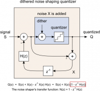
As mentioned, the previous example is one possible implementation. It's not the best possible one. But it is the first version that comes to mind. There's another common formulation which requires some more transfer function fiddeling:
The two fractions have a common denominator so they can be easily combined to one fraction. It's also possible to factor z^-1 out of the fraction:
Substituting z*(A(Z)-B(Z)) for H(z) leads to a new filter that is related to N. Note that with b0=1 it follows that z*(1-b0)=0. So, H(z) can be written as
with for . H(z) is some arbitrary filter. The big advantage now is that it is possible to plug nearly any digital filter implementation for H(z) into the noise shaping loop. One obvious approach is the difference formula from above but there are other alternatives with desirable properties. However, the purpose of this article is not to discuss digital filters in general but their application as noise shaping filters. So, throughout the rest of this article H(z) is simply treated as a black box. This black box has a certain state and gives us an output sample for each input sample. The modified pseudo code loop looks like this:
(1) h_out[k] = H.filter(last_error)
(2) wanted[k] = s[k] - h_out[k]
(3) quantized[k] = quantize( wanted[k] + dither() )
(4) last_error = quantized[k] - wanted[k]
which is equivalent to the shown signal flow graph where the unit sample delay z^-1 is implemented by the state variable 'last_error': Remember that this black box filter H(z) doesn't correspond the the actual noise shaping filter N(z). Depending on the context published coefficients for noise shaping correspond either to N(z), H(z), or -H(z).
Example filters
The following two filters have been designed by Sebastian Gesemann via non-linear optimization to match a slightly modified version of the LAME MP3 encoder's ATH (absolute threshold of hearing) curve. They were first published in the Hydrogenaudio forum including the noise transfer function's second order factorizations.
Sampling rate of 44100 Hz, derived from LAME's ATH formula
The noise transfer function is given by
The corresponding filter H is given by
Sampling rate of 48000 Hz, derived from LAME's ATH formula
The noise transfer function is given by
The corresponding filter H is given by
Notes
References
- Lipshitz. P, Stanley and John Vanderkooy. "Why 1-bit Sigma-Delta Conversion is Unsuitable for High-Quality Applications". 110th Convention. Audio Engineering Society (May 2001). 2-4.


