ReplayGain 1.0 specification: Difference between revisions
(→Equal Loudness Filter: populate with text and images) |
(more population - safety save) |
||
| Line 22: | Line 22: | ||
If every frequency sounded equally loud, then this graph would just be a series of horizontal lines. As it isn't, a filter is required to simulate this characteristic. | If every frequency sounded equally loud, then this graph would just be a series of horizontal lines. As it isn't, a filter is required to simulate this characteristic. | ||
<br style="clear:both" /> | |||
====Required equal loudness filter==== | ====Required equal loudness filter==== | ||
[[File:RG_Equal_loudness_inverse.gif|frame|Figure 2: Loudness contours inverse response]] | |||
Where the lines curve upwards, this means that we are less sensitive to sounds of that frequency. Hence, the filter must attenuate (reduce) sounds of that frequency. The ideal filter will be the inverse of the above graphs. As we don't know the replay level yet, and don't want to use a different filter for sounds of differing loudness, a representative average of the above curves will is chosen as the target filter: | Where the lines curve upwards, this means that we are less sensitive to sounds of that frequency. Hence, the filter must attenuate (reduce) sounds of that frequency. The ideal filter will be the inverse of the above graphs. As we don't know the replay level yet, and don't want to use a different filter for sounds of differing loudness, a representative average of the above curves will is chosen as the target filter: | ||
<br style="clear:both" /> | |||
====Design of the equal loudness filter==== | ====Design of the equal loudness filter==== | ||
[[File:RG_Equal_loudness_yulewalk.gif|frame|Figure 3: Target response (blue) and "yulewalk" filter response (magenta)]] | |||
[[File:RG_Equal_loudness_all.gif|frame|Figure 4: Target response (blue), high-pass response (green) and composite response (red)]] | |||
MATLAB offers several functions to design FIR and IIR filters to match arbitrary amplitude responses. Feeding the target response into yulewalk.m, and requesting a 2x10 coefficient IIR filter gives the following response: | MATLAB offers several functions to design FIR and IIR filters to match arbitrary amplitude responses. Feeding the target response into yulewalk.m, and requesting a 2x10 coefficient IIR filter gives the following response: | ||
At higher frequencies, this filter is an excellent approximation to our target. However, it lower frequencies, it doesn't even come close. Increasing the number of coefficients does not cause the yulewalk function to perform significantly better. | At higher frequencies, this filter is an excellent approximation to our target. However, it lower frequencies, it doesn't even come close. Increasing the number of coefficients does not cause the yulewalk function to perform significantly better. | ||
One solution is to cascade the yulewalk filter with a 2nd order Butterworth high pass filter, with a high pass frequency of 150 Hz. The resulting combined response is close to our target response, and is used by Replay Level | One solution is to cascade the yulewalk filter with a 2nd order Butterworth high pass filter, with a high pass frequency of 150 Hz. The resulting combined response (Figure 4) is close to our target response, and is used by Replay Level. | ||
<br style="clear:both" /> | |||
===RMS Energy Calculation=== | ===RMS Energy Calculation=== | ||
Next, the energy during each moment of the signal is determined by calculating the Root Mean Square of the waveform every 50ms. | Next, the energy during each moment of the signal is determined by calculating the Root Mean Square of the waveform every 50ms. | ||
It's easy to calculate the RMS energy over an entire audio file. For example, Cool Edit Pro (from Syntrillium) does this in its Analise:statistics box. Unfortunately, this value doesn't give a good indication of the perceived loudness of a signal. It's closer than that given by the peak amplitude, but it's still not good enough. For this reason, we have to calculate the RMS energy on a moment by moment basis (as described on this page), then do something useful with all that data. | |||
====General concept==== | |||
The signal is chopped into 50ms long blocks. Then, for each block: | |||
# Every sample value is squared (multiplied by itself). | |||
# The mean average is taken. | |||
# The square root of the average is calculated. | |||
If you read those steps backwards, it's obvious why it's called Root Mean Square (RMS) averaging. Basically, that's all we have to do. | |||
====Averaging time==== | |||
The block length of 50ms was chosen after studying the effect of values between 25ms and 1s. 25ms was too short to accurately reflect the perceived loudness of some sounds. Beyond 50ms there was little change (after statistical processing). For this reason, 50ms was chosen. | |||
====Stereo files==== | |||
The only difficulty lies in what to do with stereo files. We could sum them to mono before calculating the RMS energy, but then any out-of-phase components (having the opposite signal on each channel) would cancel out to zero (i.e. silence). That's not how we perceive them, so it's not a good solution. | |||
The alternative is to calculate two RMS values (once for each channel) and then add them. Unfortunately a Linear addition still doesn't give the same effect as our ears. To demonstrate this, consider a mono (single channel) audio track. We replay it over 1 loudspeaker, and remember how loud it sounds. If we now replay it over 2 loudspeakers, how large should the signal to each speaker be such that, overall, the sound is still as loud as before? You'd think the answer would be half as large (since we have two speakers - that's what a linear addition would suggest) but if you try it, you'll find that the answer is about 3/4. | |||
We get the right answer if we add the means of the channel-signals before calculating the square root. In mixing pan-pot terms, we're using "equal power" rather than "equal voltage". If we also assume that any mono (single channel) signal will always be replayed over two loudspeakers, we can treat a mono signal as a pair of identical stereo signals. Hence a mono signal gives (a+a)/2 (i.e. a), while a stereo signal gives (a+b)/2, where a and b are the mean squared values for each channel. After this, we carry out the square root and conversion to dB. | |||
===Statistical Processing=== | ===Statistical Processing=== | ||
[[File:RG_Statistical_speech.gif|frame|Figure 5: Histogram of classical music]] | |||
[[File:RG_Statistical_classic.gif|frame|Figure 6: Histogram of classical music]] | |||
[[File:RG_Statistical_pop.gif|frame|Figure 7: Histogram of classical music]] | |||
Where the average energy level of a signal varies with time, the louder moments contribute most to our perception of overall loudness. For example, in human speech, over half the time is silence, but this does not affect the perceived loudness of the talker at all! For this reason, the RMS values are sorted into numerical order, and the value 5% down the list is chosen to represent the overall perceived loudness of the signal. | Where the average energy level of a signal varies with time, the louder moments contribute most to our perception of overall loudness. For example, in human speech, over half the time is silence, but this does not affect the perceived loudness of the talker at all! For this reason, the RMS values are sorted into numerical order, and the value 5% down the list is chosen to represent the overall perceived loudness of the signal. | ||
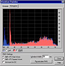
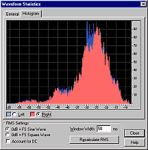
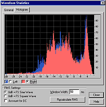
Having calculated RMS signal levels every 50ms through the file, a single value must be calculated to represent the perceived loudness of the entire file. The above histograms show how many times each RMS value occurred in each file. | |||
The most common RMS value in the speech track was -45dB (background noise) - so the most common RMS value is clearly NOT a good indicator of perceived loudness! The average RMS value is similarly misleading with the speech sample, and also with classical music. | |||
A good method to determine the overall perceived loudness is to sort the RMS energy values into numerical order, and then pick a value near the top of the list. | |||
====Choosing one represetative value==== | |||
How far down the sorted list should we look for a representative value? I tried values from 70% to 95%. For highly compressed pop music (e.g. the middle graph above, where there are many values near the top), the choice makes little difference. For speech and classical music, the choice makes a huge difference. The value which most accurately matches human perception of perceived loudness is around 95%, so this value is used by Replay Level. | |||
<br style="clear:both" /> | |||
===Calibration with reference level=== | ===Calibration with reference level=== | ||
A suitable average replay level is 83dB SPL. A calibration relating the energy of a digital signal to the real world replay level has been defined by the SMPTE. Using this calibration, we subtract the current signal from the desired (calibrated) level to give the difference. We store this difference in the audio file. | A suitable average replay level is 83dB SPL. A calibration relating the energy of a digital signal to the real world replay level has been defined by the SMPTE. Using this calibration, we subtract the current signal from the desired (calibrated) level to give the difference. We store this difference in the audio file. | ||
===Replay | ====Finding a standard==== | ||
Having calculated a representative RMS energy value for the audio file, we now need to reference this to a real world sound pressure level. The audio industry doesn't have any standard for listening level, but the movie industry has worked to an 83dB standard for years.<ref>This number (83dB SPL) wasn't picked at random. It represents a comfortable average listening level, determined by professionals from years of listening. That reference level of -20dB pink noise isn't random either. It causes the calibrated average level to be 20dB less than the peak level. In other words, it leaves 20dB of headroom for louder than average signals. So, if CDs were mastered this way, the average level would be around -20dB FS, leaving lots of room for the dramatic peaks which make music exciting.</ref> | |||
What the standard actually states is that a single channel pink noise signal, with an RMS energy level of -20 dB relative to a full scale sinusoid should be reproduced at 83 dB SPL (measured using a C-weighted, slow averaging SPL meter). In simple terms, this means that everyone can set their volume control to the same (known, calibrated) gain. | |||
====An ideal world...==== | |||
NOW (are you still with me?) if the mastering engineer set the levels on a CD using that calibrated volume control setting, that CD will sound best at that volume. If all CDs were mastered in such a way, they'd all sound best at that volume. If you (as a listener) didn't want to listen at that particular volume setting, you could always turn it down, but all CDs would still sound equalling "turned down" at your preferred setting. You wouldn't have to change the volume setting between discs. | |||
Reality check! We know CDs aren't made like this. There is NO audio standard replay level. So, here's the clever bit - here's the whole point of this website... | |||
====Fixing a non-ideal world==== | |||
We know the level should average around 83dB SPL, and we know a -20dB pink noise signal will give 83dB SPL in a calibrated system. So, we send the pink noise signal through the ReplayGain program, and store the result (let's call it ref_Vrms). For every CD we process, the difference between the calculated value for that CD and ref_Vrms tells you how much you need to scale the signal in order to make it average 83dB. | |||
The actual process is quicker to do than to say! | |||
====One complication==== | |||
The system calibration uses a single channel of pink noise (reproduced through a single loudspeaker). You then play music through both loudspeakers. So, though we use 1 channel of pink noise to calibrate the system gain, the ideal level of the music is actually the loudness when both speakers are in use. So, in ReplayGain, we calibrate to 2 channels of pink noise, because that's how loud we'd like the music to sound. In reality, we just have a monophonic pink noise wavefile, and ReplayGain automatically assumes you're playing it through both speakers, as it would any monophonic file. | |||
===Replay gain data format=== | |||
The calibration level of 83dB can be added to the difference from the previous calculation, to yield the actual Replay Gain. NOTE: we store the differential, NOT the actual Replay Gain. | The calibration level of 83dB can be added to the difference from the previous calculation, to yield the actual Replay Gain. NOTE: we store the differential, NOT the actual Replay Gain. | ||
====What to store==== | |||
Three values must be stored. | |||
# Peak signal amplitude | |||
# "Radio" = Replay Gain adjustment required to make all tracks equal loudness | |||
# "Audiophile" = Replay Gain adjustment required to give ideal listening loudness | |||
If calculated on a track-by-track basis, ReplayGain yields (2). If calculated on a disc-by-disc basis, ReplayGain will usually yield (3), though this value may be more accurately determined by a human listener if required. | |||
To allow for future expansion: If more than three values are stored, players should ignore those they do not recognise, but process those that they do. If additional Replay Gain adjustments other than "Radio" and "Audiophile" are stored, they should come after "Radio" and "Audiophile". The Peak Amplitude must always occupy the first 4 bytes of the Replay Gain header frame. The three values listed above (or at least fields to hold the three values, should the values themselves be unknown) are required in all Replay Gain headers. | |||
====Range==== | |||
The replay gain adjustment must be between -51.0dB and +51.0dB. Values outside this range must be limited to be within the range, though they are certainly in error, and should probably be re-calculated, or stored as "not set". For example, trying to cause a silent 24-bit file to play at 83dB will yield a replay gain adjustment of +57dB. | |||
In practice, adjustment values from -23dB to +17dB are the likely extremes, and values from -18dB to +2dB are more usual. | |||
====Bit format==== | |||
Each Replay Gain value should be stored in a Replay Gain Adjustment field consisting of two bytes (16 bits). Here are two example Replay Gain Adjustment fields: | |||
Radio gain adjustment | |||
<tt> | |||
0 0 1 0 1 1 1 0 0 1 1 1 1 1 0 1 | |||
\\___/ \\___/ | \\_______________/ | |||
| | | | | |||
name | sign | | |||
code | bit | | |||
| | | |||
originator | | |||
code | | |||
Replay Gain | |||
Adjustment | |||
</tt> | |||
Audiophile gain adjustment | |||
<tt> | |||
0 1 0 0 1 0 0 0 0 0 0 1 0 1 0 0 | |||
\___/ \___/ | \_______________/ | |||
| | | | | |||
name | sign | | |||
code | bit | | |||
| | | |||
originator | | |||
code | | |||
Replay Gain | |||
Adjustment | |||
</tt> | |||
==Notes== | |||
<references /> | |||
Revision as of 21:36, 11 December 2010
The Problem
Not all CDs sound equally loud. The perceived loudness of mp3s is even more variable. Whilst different musical moods require that some tracks should sound louder than others, the loudness of a given CD has more to do with the year of issue or the whim of the producer than the intended emotional effect. If we add to this chaos the inconsistent quality of mp3 encoding, it's no wonder that a random play through your music collection can have you leaping for the volume control every other track.
The solution
There is a remarkably simple solution to this annoyance, and that is to store the required replay gain for each track within the track. This concept is called "MetaData" – data about data. It's already possible to store the title, artist, and CD track number within an mp3 file using the ID3 standard. The later ID3v2 standard also incorporates the ability to store a track relative volume adjustment, which can be used to "fix" quiet or loud sounding mp3s.
However, there is no consistent standard by which to define the appropriate replay gain which mp3 encoders and players agree on, and no automatic way to set the volume adjustment for each track – until now.
The Replay Gain proposal sets out a simple way of calculating and representing the ideal replay gain for every track and album.
Calculation
Equal Loudness Filter
The human ear does not perceive sounds of all frequencies as having equal loudness. For example, a full scale sine wave at 1kHz sounds much louder than a full scale sine wave at 10kHz, even though the two have identical energy. To account for this, the signal is filtered by an inverted approximation to the equal loudness curves (sometimes referred to as Fletcher-Munson curves).
Equal loudness curves
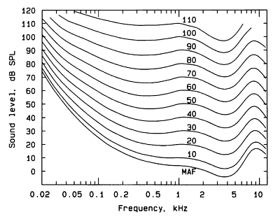
Figure 1 shows the Equal Loudness Contours, as measured by Robinson and Dadson, 1956. The original measurements were carried out by Fletcher and Munson in 1933, and the curve often carries their name.
The lines represent the sound pressure required for a test tone of any frequency to sound as loud as a test tone of 1 kHz. Take the line marked "60" - at 1 kHz ("1" on the x axis), the line marked "60" is at 60dB (on the y axis). If you follow the "60" line down to 0.5 kHz (500 Hz), and look across to the y axis, the value is about 55 dB. What this means is that a 500 Hz tone at 55 dB SPL sounds as loud to a human listener as a 1 kHz tone at 60 dB SPL.
If every frequency sounded equally loud, then this graph would just be a series of horizontal lines. As it isn't, a filter is required to simulate this characteristic.
Required equal loudness filter
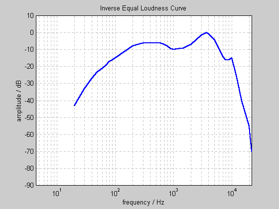
Where the lines curve upwards, this means that we are less sensitive to sounds of that frequency. Hence, the filter must attenuate (reduce) sounds of that frequency. The ideal filter will be the inverse of the above graphs. As we don't know the replay level yet, and don't want to use a different filter for sounds of differing loudness, a representative average of the above curves will is chosen as the target filter:
Design of the equal loudness filter
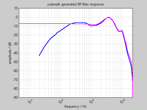
MATLAB offers several functions to design FIR and IIR filters to match arbitrary amplitude responses. Feeding the target response into yulewalk.m, and requesting a 2x10 coefficient IIR filter gives the following response:
At higher frequencies, this filter is an excellent approximation to our target. However, it lower frequencies, it doesn't even come close. Increasing the number of coefficients does not cause the yulewalk function to perform significantly better.
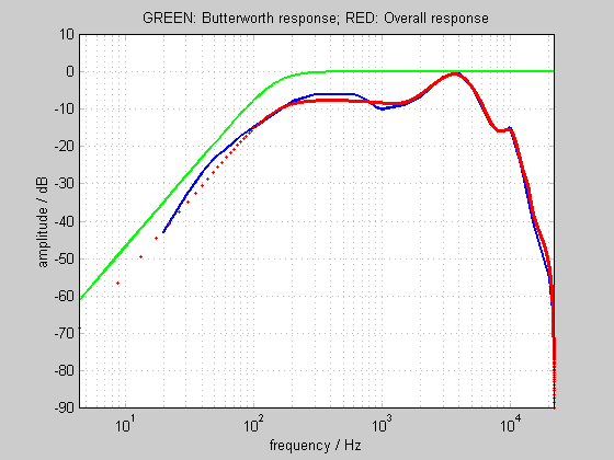
One solution is to cascade the yulewalk filter with a 2nd order Butterworth high pass filter, with a high pass frequency of 150 Hz. The resulting combined response (Figure 4) is close to our target response, and is used by Replay Level.
RMS Energy Calculation
Next, the energy during each moment of the signal is determined by calculating the Root Mean Square of the waveform every 50ms.
It's easy to calculate the RMS energy over an entire audio file. For example, Cool Edit Pro (from Syntrillium) does this in its Analise:statistics box. Unfortunately, this value doesn't give a good indication of the perceived loudness of a signal. It's closer than that given by the peak amplitude, but it's still not good enough. For this reason, we have to calculate the RMS energy on a moment by moment basis (as described on this page), then do something useful with all that data.
General concept
The signal is chopped into 50ms long blocks. Then, for each block:
- Every sample value is squared (multiplied by itself).
- The mean average is taken.
- The square root of the average is calculated.
If you read those steps backwards, it's obvious why it's called Root Mean Square (RMS) averaging. Basically, that's all we have to do.
Averaging time
The block length of 50ms was chosen after studying the effect of values between 25ms and 1s. 25ms was too short to accurately reflect the perceived loudness of some sounds. Beyond 50ms there was little change (after statistical processing). For this reason, 50ms was chosen.
Stereo files
The only difficulty lies in what to do with stereo files. We could sum them to mono before calculating the RMS energy, but then any out-of-phase components (having the opposite signal on each channel) would cancel out to zero (i.e. silence). That's not how we perceive them, so it's not a good solution.
The alternative is to calculate two RMS values (once for each channel) and then add them. Unfortunately a Linear addition still doesn't give the same effect as our ears. To demonstrate this, consider a mono (single channel) audio track. We replay it over 1 loudspeaker, and remember how loud it sounds. If we now replay it over 2 loudspeakers, how large should the signal to each speaker be such that, overall, the sound is still as loud as before? You'd think the answer would be half as large (since we have two speakers - that's what a linear addition would suggest) but if you try it, you'll find that the answer is about 3/4.
We get the right answer if we add the means of the channel-signals before calculating the square root. In mixing pan-pot terms, we're using "equal power" rather than "equal voltage". If we also assume that any mono (single channel) signal will always be replayed over two loudspeakers, we can treat a mono signal as a pair of identical stereo signals. Hence a mono signal gives (a+a)/2 (i.e. a), while a stereo signal gives (a+b)/2, where a and b are the mean squared values for each channel. After this, we carry out the square root and conversion to dB.
Statistical Processing
Where the average energy level of a signal varies with time, the louder moments contribute most to our perception of overall loudness. For example, in human speech, over half the time is silence, but this does not affect the perceived loudness of the talker at all! For this reason, the RMS values are sorted into numerical order, and the value 5% down the list is chosen to represent the overall perceived loudness of the signal.
Having calculated RMS signal levels every 50ms through the file, a single value must be calculated to represent the perceived loudness of the entire file. The above histograms show how many times each RMS value occurred in each file.
The most common RMS value in the speech track was -45dB (background noise) - so the most common RMS value is clearly NOT a good indicator of perceived loudness! The average RMS value is similarly misleading with the speech sample, and also with classical music.
A good method to determine the overall perceived loudness is to sort the RMS energy values into numerical order, and then pick a value near the top of the list.
Choosing one represetative value
How far down the sorted list should we look for a representative value? I tried values from 70% to 95%. For highly compressed pop music (e.g. the middle graph above, where there are many values near the top), the choice makes little difference. For speech and classical music, the choice makes a huge difference. The value which most accurately matches human perception of perceived loudness is around 95%, so this value is used by Replay Level.
Calibration with reference level
A suitable average replay level is 83dB SPL. A calibration relating the energy of a digital signal to the real world replay level has been defined by the SMPTE. Using this calibration, we subtract the current signal from the desired (calibrated) level to give the difference. We store this difference in the audio file.
Finding a standard
Having calculated a representative RMS energy value for the audio file, we now need to reference this to a real world sound pressure level. The audio industry doesn't have any standard for listening level, but the movie industry has worked to an 83dB standard for years.[1]
What the standard actually states is that a single channel pink noise signal, with an RMS energy level of -20 dB relative to a full scale sinusoid should be reproduced at 83 dB SPL (measured using a C-weighted, slow averaging SPL meter). In simple terms, this means that everyone can set their volume control to the same (known, calibrated) gain.
An ideal world...
NOW (are you still with me?) if the mastering engineer set the levels on a CD using that calibrated volume control setting, that CD will sound best at that volume. If all CDs were mastered in such a way, they'd all sound best at that volume. If you (as a listener) didn't want to listen at that particular volume setting, you could always turn it down, but all CDs would still sound equalling "turned down" at your preferred setting. You wouldn't have to change the volume setting between discs.
Reality check! We know CDs aren't made like this. There is NO audio standard replay level. So, here's the clever bit - here's the whole point of this website...
Fixing a non-ideal world
We know the level should average around 83dB SPL, and we know a -20dB pink noise signal will give 83dB SPL in a calibrated system. So, we send the pink noise signal through the ReplayGain program, and store the result (let's call it ref_Vrms). For every CD we process, the difference between the calculated value for that CD and ref_Vrms tells you how much you need to scale the signal in order to make it average 83dB.
The actual process is quicker to do than to say!
One complication
The system calibration uses a single channel of pink noise (reproduced through a single loudspeaker). You then play music through both loudspeakers. So, though we use 1 channel of pink noise to calibrate the system gain, the ideal level of the music is actually the loudness when both speakers are in use. So, in ReplayGain, we calibrate to 2 channels of pink noise, because that's how loud we'd like the music to sound. In reality, we just have a monophonic pink noise wavefile, and ReplayGain automatically assumes you're playing it through both speakers, as it would any monophonic file.
Replay gain data format
The calibration level of 83dB can be added to the difference from the previous calculation, to yield the actual Replay Gain. NOTE: we store the differential, NOT the actual Replay Gain.
What to store
Three values must be stored.
- Peak signal amplitude
- "Radio" = Replay Gain adjustment required to make all tracks equal loudness
- "Audiophile" = Replay Gain adjustment required to give ideal listening loudness
If calculated on a track-by-track basis, ReplayGain yields (2). If calculated on a disc-by-disc basis, ReplayGain will usually yield (3), though this value may be more accurately determined by a human listener if required.
To allow for future expansion: If more than three values are stored, players should ignore those they do not recognise, but process those that they do. If additional Replay Gain adjustments other than "Radio" and "Audiophile" are stored, they should come after "Radio" and "Audiophile". The Peak Amplitude must always occupy the first 4 bytes of the Replay Gain header frame. The three values listed above (or at least fields to hold the three values, should the values themselves be unknown) are required in all Replay Gain headers.
Range
The replay gain adjustment must be between -51.0dB and +51.0dB. Values outside this range must be limited to be within the range, though they are certainly in error, and should probably be re-calculated, or stored as "not set". For example, trying to cause a silent 24-bit file to play at 83dB will yield a replay gain adjustment of +57dB.
In practice, adjustment values from -23dB to +17dB are the likely extremes, and values from -18dB to +2dB are more usual.
Bit format
Each Replay Gain value should be stored in a Replay Gain Adjustment field consisting of two bytes (16 bits). Here are two example Replay Gain Adjustment fields:
Radio gain adjustment
0 0 1 0 1 1 1 0 0 1 1 1 1 1 0 1 \\___/ \\___/ | \\_______________/
| | | |
name | sign | code | bit |
       |             |
  originator         |
     code            |
                Replay Gain
                 Adjustment
Audiophile gain adjustment 0 1 0 0 1 0 0 0 0 0 0 1 0 1 0 0 \___/ \___/ | \_______________/
| | | |
name | sign | code | bit |
       |             |
  originator         |
     code            |
                Replay Gain
                 Adjustment
Notes
- ↑ This number (83dB SPL) wasn't picked at random. It represents a comfortable average listening level, determined by professionals from years of listening. That reference level of -20dB pink noise isn't random either. It causes the calibrated average level to be 20dB less than the peak level. In other words, it leaves 20dB of headroom for louder than average signals. So, if CDs were mastered this way, the average level would be around -20dB FS, leaving lots of room for the dramatic peaks which make music exciting.
