ReplayGain 1.0 specification

The Problem

Not all CDs sound equally loud. The perceived loudness of mp3s is even more variable. Whilst different musical moods require that some tracks should sound louder than others, the loudness of a given CD has more to do with the year of issue or the whim of the producer than the intended emotional effect. If we add to this chaos the inconsistent quality of mp3 encoding, it's no wonder that a random play through your music collection can have you leaping for the volume control every other track.

The solution

There is a remarkably simple solution to this annoyance, and that is to store the required replay gain for each track within the track. This concept is called "MetaData" – data about data. It's already possible to store the title, artist, and CD track number within an mp3 file using the ID3 standard. The later ID3v2 standard also incorporates the ability to store a track relative volume adjustment, which can be used to "fix" quiet or loud sounding mp3s.

However, there is no consistent standard by which to define the appropriate replay gain which mp3 encoders and players agree on, and no automatic way to set the volume adjustment for each track – until now.

The Replay Gain proposal sets out a simple way of calculating and representing the ideal replay gain for every track and album.

Calculation

Equal Loudness Filter

The human ear does not perceive sounds of all frequencies as having equal loudness. For example, a full scale sine wave at 1kHz sounds much louder than a full scale sine wave at 10kHz, even though the two have identical energy. To account for this, the signal is filtered by an inverted approximation to the equal loudness curves (sometimes referred to as Fletcher-Munson curves).

Equal loudness curves

Figure 1: Equal loudness contours

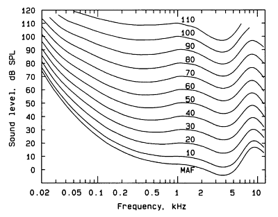
Figure 1 shows the Equal Loudness Contours, as measured by Robinson and Dadson, 1956. The original measurements were carried out by Fletcher and Munson in 1933, and the curve often carries their name.

The lines represent the sound pressure required for a test tone of any frequency to sound as loud as a test tone of 1 kHz. Take the line marked "60" - at 1 kHz ("1" on the x axis), the line marked "60" is at 60dB (on the y axis). If you follow the "60" line down to 0.5 kHz (500 Hz), and look across to the y axis, the value is about 55 dB. What this means is that a 500 Hz tone at 55 dB SPL sounds as loud to a human listener as a 1 kHz tone at 60 dB SPL.

If every frequency sounded equally loud, then this graph would just be a series of horizontal lines. As it isn't, a filter is required to simulate this characteristic.

Required equal loudness filter

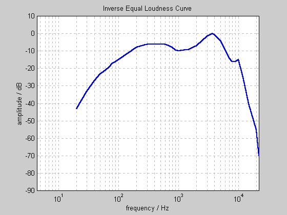
Where the lines curve upwards, this means that we are less sensitive to sounds of that frequency. Hence, the filter must attenuate (reduce) sounds of that frequency. The ideal filter will be the inverse of the above graphs. As we don't know the replay level yet, and don't want to use a different filter for sounds of differing loudness, a representative average of the above curves will is chosen as the target filter:

Loudness contours inverse response

Design of the equal loudness filter

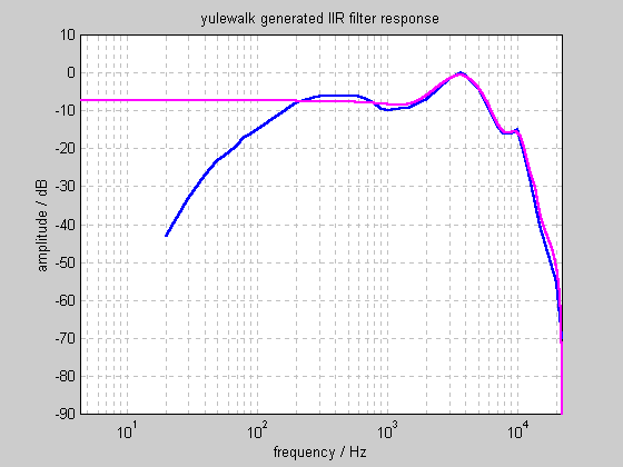
MATLAB offers several functions to design FIR and IIR filters to match arbitrary amplitude responses. Feeding the target response into yulewalk.m, and requesting a 2x10 coefficient IIR filter gives the following response:

Target response (blue) and "yulewalk" filter response (magenta)

At higher frequencies, this filter is an excellent approximation to our target. However, it lower frequencies, it doesn't even come close. Increasing the number of coefficients does not cause the yulewalk function to perform significantly better.

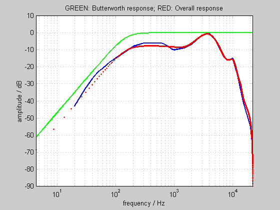
One solution is to cascade the yulewalk filter with a 2nd order Butterworth high pass filter, with a high pass frequency of 150 Hz. The resulting combined response is close to our target response, and is used by Replay Level:

Target response (blue), high-pass response (green) and composite response (red)

RMS Energy Calculation

Next, the energy during each moment of the signal is determined by calculating the Root Mean Square of the waveform every 50ms.

Statistical Processing

Where the average energy level of a signal varies with time, the louder moments contribute most to our perception of overall loudness. For example, in human speech, over half the time is silence, but this does not affect the perceived loudness of the talker at all! For this reason, the RMS values are sorted into numerical order, and the value 5% down the list is chosen to represent the overall perceived loudness of the signal.

Calibration with reference level

A suitable average replay level is 83dB SPL. A calibration relating the energy of a digital signal to the real world replay level has been defined by the SMPTE. Using this calibration, we subtract the current signal from the desired (calibrated) level to give the difference. We store this difference in the audio file.

Replay Gain

The calibration level of 83dB can be added to the difference from the previous calculation, to yield the actual Replay Gain. NOTE: we store the differential, NOT the actual Replay Gain.